Layer 5 — AutoCorrelation 精读

由 AutoCorrelationLayer.forward() 调用（[[04-Layer4-AutoCorrelationLayer]]）。
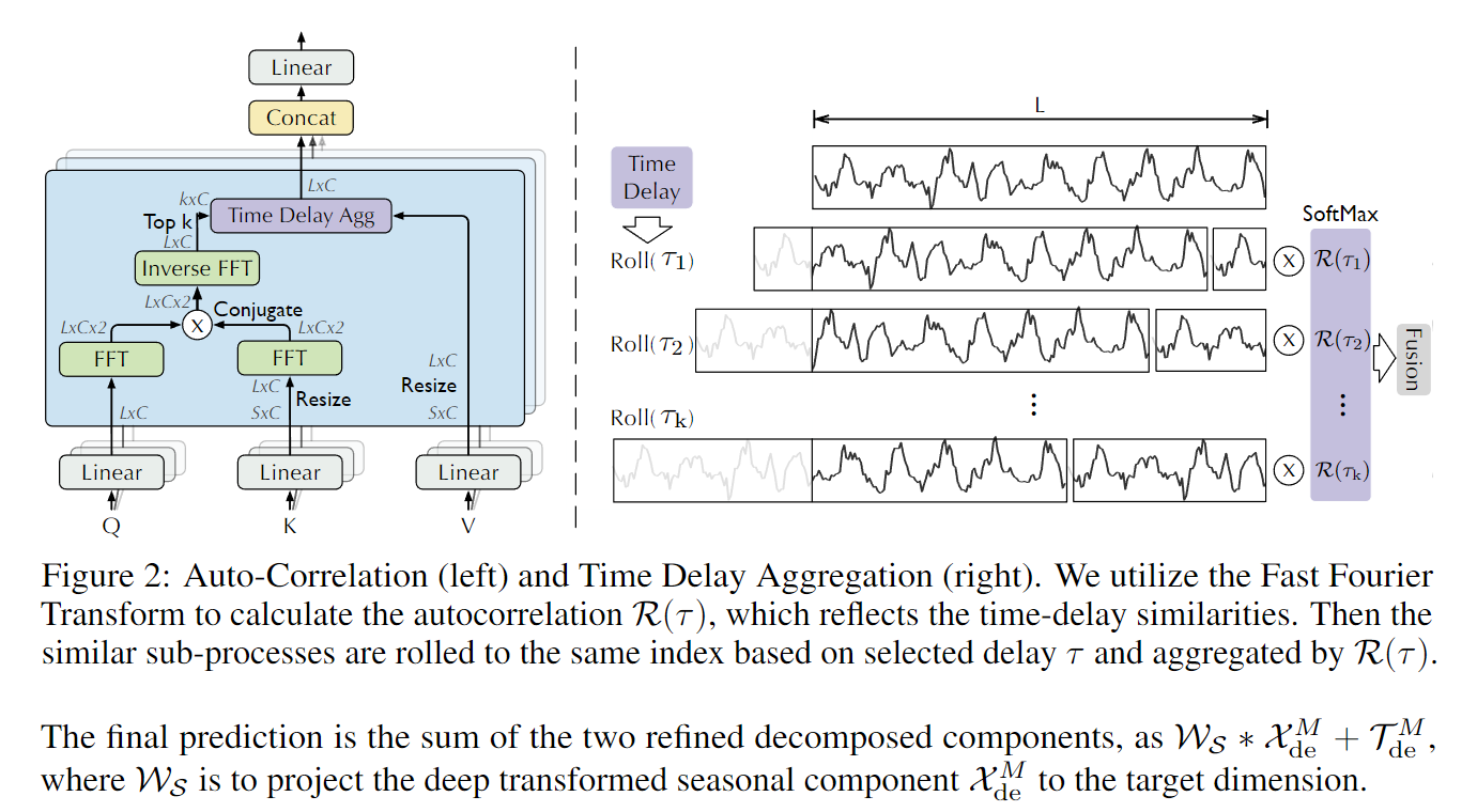
本层是 Autoformer 的核心创新：FFT 互相关发现主导 lag，时延聚合替代点积注意力。

---

1. 在父层中的位置

AutoCorrelationLayer.forward()
  └─ self.inner_correlation(queries, keys, values, attn_mask)  ← AutoCorrelation（本文档）

---

2. I/O 接口定义

以 EncoderLayer 自注意力（toy，encoder seq_len=12）为例：

	shape	含义
输入 queries	(2, 12, 4, 2) = (B, L, H, E)	多头 Q
输入 keys	(2, 12, 4, 2) = (B, S, H, E)	多头 K
输入 values	(2, 12, 4, 2) = (B, S, H, D)	多头 V
输出 V	(2, 12, 4, 2) = (B, L, H, D)	时延聚合后的上下文向量
输出 attn	None	output_attention=False 时为 None

---

3. 顺序图（具体层）

---

4. 语义分组图（索引层）

---

5. 逐步精读

5.0 完整原始代码

class AutoCorrelation(nn.Module):
    """
    AutoCorrelation Mechanism with the following two phases:
    (1) period-based dependencies discovery
    (2) time delay aggregation
    This block can replace the self-attention family mechanism seamlessly.
    """

    def __init__(
        self,
        mask_flag=True,
        factor=1,
        scale=None,
        attention_dropout=0.1,
        output_attention=False,
    ):
        super(AutoCorrelation, self).__init__()
        self.factor = factor
        self.scale = scale
        self.mask_flag = mask_flag
        self.output_attention = output_attention
        self.dropout = nn.Dropout(attention_dropout)
	        
	def forward(self, queries, keys, values, attn_mask):
	    B, L, H, E = queries.shape
	    _, S, _, D = values.shape
	    if L > S:
	        zeros = torch.zeros_like(queries[:, : (L - S), :]).float()
	        values = torch.cat([values, zeros], dim=1)
	        keys = torch.cat([keys, zeros], dim=1)
	    else:
	        values = values[:, :L, :, :]
	        keys = keys[:, :L, :, :]
	
	    # period-based dependencies
	    q_fft = torch.fft.rfft(queries.permute(0, 2, 3, 1).contiguous(), dim=-1)
	    k_fft = torch.fft.rfft(keys.permute(0, 2, 3, 1).contiguous(), dim=-1)
	    res = q_fft * torch.conj(k_fft)
	    corr = torch.fft.irfft(res, dim=-1)
	
	    # time delay agg
	    if self.training:
	        V = self.time_delay_agg_training(
	            values.permute(0, 2, 3, 1).contiguous(), corr
	        ).permute(0, 3, 1, 2)
	    else:
	        V = self.time_delay_agg_inference(
	            values.permute(0, 2, 3, 1).contiguous(), corr
	        ).permute(0, 3, 1, 2)
	
	    if self.output_attention:
	        return (V.contiguous(), corr.permute(0, 3, 1, 2))
	    else:
	        return (V.contiguous(), None)

---

5.1 宏观逻辑：AutoCorrelation 的计算公式链

标准注意力的计算流水线是：

$$\text{scores}=\frac{Q{K}^T}{\sqrt{E}}\stackrel{\text{softmax}}{\to }\alpha \stackrel{\cdot V}{\to }\text{Out}$$

AutoCorrelation 的流水线对应地是：

$$Q,K\stackrel{\text{FFT 互相关}}{\to }\text{corr}[\tau ]\stackrel{\text{top-k + softmax}}{\to }{w}_k,{\tau }_k\stackrel{\text{roll}(V,-{\tau }_k)\text{ 加权叠加}}{\to }\text{Out}$$

下面逐段推导每一步的数学含义和实现方式。

---

第一步：用互相关代替点积 — 计算 corr[τ]

点积注意力 $Q_i\cdot K_j$ 量化的是"位置 i 和位置 j 的向量有多相似"。

互相关函数 $C[\tau ]$ 量化的是"Q 和 K 在时间偏移 τ 下有多对齐"：

$$C_{QK}(\tau )=\sum _{t=0}^{L-1}Q[t]\cdot K[(t+\tau )modL]$$

直觉：把 K 整体右移 τ 步，再与 Q 逐位点积求和。τ 是周期 lag，当 τ 等于序列真实周期时，移位后的 K 和 Q 完美对齐，C[τ] 取得峰值。

用一条周期=4 的信号 Q = K = [1,3,2,4, 1,3,2,4, 1,3,2,4] 验证：

τ=0: K 右移0 = [1,3,2,4,1,3,2,4,1,3,2,4]  → C[0] = 1²+3²+2²+4²+... = 60
τ=1: K 右移1 = [4,1,3,2,4,1,3,2,4,1,3,2]  → C[1] = 1×4+3×1+2×3+...   ← 错位，值小
τ=4: K 右移4 = [1,3,2,4,1,3,2,4,1,3,2,4]  → C[4] = 60（和τ=0一样！完美对齐）
τ=8: 同理 → C[8] = 60

C 的峰值在 τ=0,4,8，正好是周期的整数倍。这就是 corr 张量在计算的东西：每个 τ 位置存一个"该偏移量下的全局对齐强度"。

代码里怎么算：直接按定义算要 $O(L^2)$（L 个 τ，每个 τ 需要 L 次乘法）。用互相关定理加速：

$$C_{QK}=\text{IFFT}(\text{FFT}(Q)\times \overline{\text{FFT}(K)})$$

$\bar{\cdot }$ 是复共轭，$\times$ 是逐元素相乘。FFT 把时域卷积变成频域乘法，整体 $O(L\log L)$。代码直接实现此定理：

q_fft = torch.fft.rfft(queries_time_major, dim=-1)   # (B,H,E,L//2+1) 复数
k_fft = torch.fft.rfft(keys_time_major,   dim=-1)
res   = q_fft * torch.conj(k_fft)                    # 逐元素复数乘法
corr  = torch.fft.irfft(res, n=L, dim=-1)            # 还原 → (B,H,E,L) 实数

rfft 利用实数信号的对称性只保留 $L//2+1$ 个频率分量（节省一半存储），irfft 还原时需显式传 n=L 告知目标长度。

---

第二步：top-k 选主周期 — 对应 softmax 之前的 score 筛选（Time Delay Agg）

得到 corr (B,H,E,L) 之后，每个 τ 都有一个相关值。直接对全部 L 个 τ 做 softmax 然后加权，代价是 $O(L)$ 个 roll 操作，且大部分 τ 的权重接近 0（噪声）。

代码取 $\text{top\_k}=\lfloor \ln L\rfloor$ 个最强 lag：

top_k = int(self.factor * math.log(length))

math.log 是自然对数 ln，ln(12) ≈ 2.48 → top_k=2。

corr 有 4 个维度 (B,H,E,L)，取 top-k 时先对 H 和 E 维度求均值，得到每个 τ 的跨头、跨通道平均强度，再在 L 维度上找最大的 k 个下标：

$$\overline{C}[\tau ]=\frac{1}{H\cdot E}\sum _{h,e}C[b,h,e,\tau ]$$

mean_value = torch.mean(torch.mean(corr, dim=1), dim=1)   # (B,L)
index      = torch.topk(torch.mean(mean_value, dim=0), top_k, dim=-1)[1]

torch.mean(mean_value, dim=0) 再对 batch 求均值 → 训练时所有样本共享同一组 top-k lag 下标（§5.4 详解）。

---

第三步：softmax 归一化 — 把互相关值变成权重（Time Delay Agg）

选出 top-k 个 lag 对应的 corr 值，softmax 归一化得到加权系数：

$$w_k=\frac{\exp (C[{\tau }_k])}{\sum _{k^{\prime }}\exp (C[{\tau }_{k^{\prime }}])}$$

对应点积注意力里的 ${\alpha }_{ij}=\text{softmax}({\text{scores}}_{ij})$，区别在于这里的下标从"位置对 (i,j)"变成了"lag 下标 k"，维度从 $(L\times L)$ 降到了 top_k。

tmp_corr = torch.softmax(torch.stack([...], dim=-1), dim=-1)   # (B, top_k)

---

第四步：roll(V, -τ) 加权叠加 — 对应 α·V（Time Delay Agg）

点积注意力的聚合：

$$\text{Out}[t]=\sum _{j=0}^{L-1}{\alpha }_{tj}\cdot V[j]$$

对每个 query 位置 t 单独算一行权重，再加权 V。这是"逐位置"聚合，输出的每个时间步看的是不同的 V 子集。

AutoCorrelation 的聚合：

$$\text{Out}=\sum _{k=1}^{\text{top\_k}}{w}_k\cdot \text{roll}(V,-{\tau }_k)$$

roll(V, -τ) 是循环左移：位置 t 上的值变成原来的 $V[(t+\tau )modL]$。

为什么是 roll 而不是 gather 特定位置：互相关发现"lag=τ 时整条序列对齐"，意味着对每一个时间步 t，需要聚合的不是某个固定位置 j，而是"当前位置 t 的 τ 步之后"——即 $V[(t+\tau )modL]$。这个 t 是变动的，对不同时间步操作的是不同的 V 下标，整体正好等于把 V 左移 τ。

展开 Out[t] 的含义：

$$\text{Out}[t]=\sum _k{w}_k\cdot V[(t+{\tau }_k)modL]$$

每个时间步 t 聚合的是"在主周期 τ_k 步之后的 V 向量"——利用的是时序的周期重复性，而非任意两位置间的语义相似性。

---

完整公式对照

步骤	标准注意力	AutoCorrelation
相似度计算	$S_{ij}=Q_i\cdot K_j/\sqrt{E}$，形状 $(L\times L)$	$C[\tau ]=\text{IFFT}(\text{FFT}(Q)\cdot \overline{\text{FFT}(K)})$，形状 $(L,)$
筛选	无筛选，全部 L² 个得分	top-k：保留 $\lfloor \ln L\rfloor$ 个最强 lag
归一化	$\alpha =\text{softmax}(S)$	$w_k=\text{softmax}(C[{\tau }_k])$
聚合	$\text{Out}[t]=\sum _j{\alpha }_{tj}{V}_j$	$\text{Out}=\sum _k{w}_k\cdot \text{roll}(V,-{\tau }_k)$

---

shape 变化链：

Q, K, V 输入：(B,L,H,E) = (2,12,4,2)
→ permute(0,2,3,1) → (2,4,2,12)
→ rfft(dim=-1)     → (2,4,2,7)      复数，L//2+1=7
→ q_fft × conj(k_fft) → (2,4,2,7)  逐元素复数乘法
→ irfft(n=12)      → corr (2,4,2,12) 每个 τ 的互相关值
→ 均值+topk        → index (top_k=2,) lag 下标
→ softmax          → w (2,2)         lag 权重
→ roll(V)+加权叠加 → Out (2,12,4,2)

math.log 为自然对数 ln（非 log₂），ln(12) ≈ 2.48 → int() 截断 → top_k=2。

---

5.2 步骤一：L/S 对齐

if L > S:
    zeros = torch.zeros_like(queries[:, : (L - S), :]).float()
    values = torch.cat([values, zeros], dim=1)
    keys = torch.cat([keys, zeros], dim=1)
else:
    values = values[:, :L, :, :]
    keys = keys[:, :L, :, :]

FFT 互相关要求 Q 和 K/V 的序列长度一致。

场景	L vs S	处理
Encoder 自注意力	L=S=12	else: values[:, :12, :, :]（无变化）
Decoder cross-attn	L=10 < S=12	else: values[:, :10, :, :]（截断 K/V 到 L）
L > S（少见）	L > S	对 K/V 末尾补零

cross-attention 截断后：keys/values 变为 (2, 10, 4, 2)，FFT 在 L=10 维度上计算。

toy 数值：Encoder 自注意力 L=S=12，无操作。

---

5.3 Phase 1 — FFT 周期发现

q_fft = torch.fft.rfft(queries.permute(0, 2, 3, 1).contiguous(), dim=-1)
k_fft = torch.fft.rfft(keys.permute(0, 2, 3, 1).contiguous(), dim=-1)
res = q_fft * torch.conj(k_fft)
corr = torch.fft.irfft(res, dim=-1)

permute 解析：
queries (B,L,H,E) → permute(0,2,3,1) → (B,H,E,L) = (2,4,2,12)
FFT 作用在最后一维（L=12），对每个 (b,h,e) 的长度12序列做变换。

rfft vs fft：
实数输入的 FFT 输出关于中心频率共轭对称。rfft 只返回非冗余的前半部分：L//2+1 = 7 个复数。

$$Q_{\text{fft}}[b,h,e,f]=\sum _{t=0}^{11}Q[b,h,e,t]\cdot e^{-2\pi ift/12}$$

互相关：
$\text{res}=Q_{\text{fft}}\times \overline{K_{\text{fft}}}$（逐元素）
这正是互相关定理：时域互相关 ↔ 频域共轭乘积。

$\text{corr}[b,h,e,\tau ]=\sum _{t}Q[b,h,e,t]\cdot K[b,h,e,(t+\tau )modL]$

toy 数值 — 最小示例（L=8）逐步推导

以下用 L=8 的短序列说明 FFT 互相关的具体计算；实际 toy 为 L=12，步骤相同，只是规模更大。

设 batch=0, head=0, e=0 的单条序列：q = k = [1, 0, 0, 0, 1, 0, 0, 0]（脉冲间隔=4，周期 p=4）

Step 1：rfft — 实数 FFT，输出 L//2+1 = 5 个复数

$$\text{q\_fft}[f]=\sum _{t=0}^{7}q[t]\cdot e^{-2\pi ift/8}$$

非零项只有 t=0 和 t=4：$\text{q\_fft}[f]=1+e^{-2\pi if\cdot 4/8}=1+e^{-\pi if}$

f	$e^{-\pi if}$	q_fft[f]
0	+1	2+0j
1	−1	0+0j
2	+1	2+0j
3	−1	0+0j
4	+1	2+0j

$\text{q\_fft}=[2+0j,0+0j,2+0j,0+0j,2+0j]$

f=2 处有能量，对应周期 $L/f=8/2=4$ ← 主周期 p=4 被正确捕捉 ✓

Step 2：res = q_fft × conj(k_fft)（自注意力 Q=K）

$$\text{res}=[4+0j,0+0j,4+0j,0+0j,4+0j]$$

Step 3：irfft(res, n=8) → corr，形状还原为 (L=8,)

irfft 补全对称频谱 $[4,0,4,0,4,0,4,0]$，再做逆变换：

$$\text{corr}[n]=\frac{1}{8}\sum _{k=0}^7\text{res\_full}[k]\cdot e^{2\pi ikn/8}$$

只有 k=0,2,4,6 非零（均为4），故 $\text{corr}[n]=\frac{4}{8}\sum _{j=0}^3{e}^{\pi ijn/2}$：

τ	corr[τ]	解读
0	2	lag=0：序列与自身完全对齐，最大正相关
1	0	无相关
2	0	无相关
3	0	无相关
4	2	lag=4：移位一个完整周期 p=4 后完全对齐 ✓
5–7	0	无相关

$$\text{corr}=[2,0,0,0,2,0,0,0]$$

top_k = $\lfloor \ln (8)\rfloor =\lfloor 2.08\rfloor =2$ → 选 lag=0 和 lag=4（即主周期）

对照实际 toy L=12：rfft 输出 $12//2+1=7$ 个复数；top_k = $\lfloor \ln (12)\rfloor =\lfloor 2.48\rfloor =2$；corr 形状 (2,4,2,12)，每个 [b,h,e,τ] 位置表示延迟 τ 步后 Q 与 K 的互相关强度。

---

5.4 Phase 2 — 时延聚合（training 路径）

def time_delay_agg_training(self, values, corr):
    head = values.shape[1]
    channel = values.shape[2]
    length = values.shape[3]
    # find top k
    top_k = int(self.factor * math.log(length))
    mean_value = torch.mean(torch.mean(corr, dim=1), dim=1)
    index = torch.topk(torch.mean(mean_value, dim=0), top_k, dim=-1)[1]
    weights = torch.stack([mean_value[:, index[i]] for i in range(top_k)], dim=-1)
    # update corr
    tmp_corr = torch.softmax(weights, dim=-1)
    # aggregation
    tmp_values = values
    delays_agg = torch.zeros_like(values).float()
    for i in range(top_k):
        pattern = torch.roll(tmp_values, -int(index[i]), -1)
        delays_agg = delays_agg + pattern * (
            tmp_corr[:, i]
            .unsqueeze(1)
            .unsqueeze(1)
            .unsqueeze(1)
            .repeat(1, head, channel, length)
        )
    return delays_agg

此处 values 已经是 permute 后的格式

调用处：values.permute(0, 2, 3, 1).contiguous()
所以传入 time_delay_agg_training 的 values 是 (B, H, D, L) = (2, 4, 2, 12)，
head=4, channel=2, length=12。

toy 输入定义

corr 是 Phase 1 的输出，shape (B, H, E, L) = (2, 4, 2, 12)。为简化追踪，设所有 head 和 channel 共享相同的 lag 强度曲线（batch 间不同）：

# batch=0：lag=2 主导，lag=5 次之
corr[0, h, e, :] = [0.20, 0.10, 2.40, 0.10, 0.20, 1.60, 0.10, 0.20, 0.10, 0.10, 0.10, 0.10]
                    τ=0   τ=1   τ=2   τ=3   τ=4   τ=5   τ=6   τ=7   τ=8   τ=9  τ=10  τ=11

# batch=1：lag=2 主导，lag=7 次之
corr[1, h, e, :] = [0.20, 0.10, 2.00, 0.10, 0.10, 0.20, 0.10, 1.80, 0.10, 0.10, 0.10, 0.10]

values[0, 0, 0, :] = [0.1, 0.3, 0.5, 0.2, 0.4, 0.6, 0.1, 0.3, 0.5, 0.2, 0.4, 0.6]（追踪切片）

---

Step 1 — 两次均值：corr → mean_value

mean_value = torch.mean(torch.mean(corr, dim=1), dim=1)

第一次 torch.mean(corr, dim=1)：对 H=4 个 head 求均值。

$$\text{corr}(2,4,2,12)\stackrel{\text{mean dim=1}}{\to }(2,2,12)$$

由于各 head 值相同，均值不变：

结果[0, e, :] = [0.20, 0.10, 2.40, 0.10, 0.20, 1.60, 0.10, 0.20, 0.10, 0.10, 0.10, 0.10]  (e=0,1)
结果[1, e, :] = [0.20, 0.10, 2.00, 0.10, 0.10, 0.20, 0.10, 1.80, 0.10, 0.10, 0.10, 0.10]  (e=0,1)

第二次 torch.mean(..., dim=1)：对 E=2 个 channel 求均值（此时 dim=1 对应 E 维）。

$$\stackrel{\text{mean dim=1}}{\to }(2,12)=\text{mean\_value}$$

由于两个 channel 值相同，均值仍不变：

mean_value[0, :] = [0.20, 0.10, 2.40, 0.10, 0.20, 1.60, 0.10, 0.20, 0.10, 0.10, 0.10, 0.10]
mean_value[1, :] = [0.20, 0.10, 2.00, 0.10, 0.10, 0.20, 0.10, 1.80, 0.10, 0.10, 0.10, 0.10]

mean_value[b, τ] = 样本 b 在延迟 τ 时的平均互相关强度（已跨所有 head 和 channel 压缩）。

---

Step 2 — batch 均值 → topk：全局共享 index

index = torch.topk(torch.mean(mean_value, dim=0), top_k, dim=-1)[1]

torch.mean(mean_value, dim=0)：在 B=2 维求均值，(2,12) → (12,)：

τ=0:  (0.20+0.20)/2 = 0.20
τ=1:  (0.10+0.10)/2 = 0.10
τ=2:  (2.40+2.00)/2 = 2.20  ← 最大
τ=3:  0.10
τ=4:  (0.20+0.10)/2 = 0.15
τ=5:  (1.60+0.20)/2 = 0.90
τ=6:  0.10
τ=7:  (0.20+1.80)/2 = 1.00  ← 第二大
τ=8~11: 0.10

torch.topk(k=2)[1] 取下标 → index = tensor([2, 7])

这里体现了 Training 的"batch-norm 风格"代价

batch=0 自己最偏好的 top-2 是 [τ=2, τ=5]（2.40, 1.60）；
batch=1 自己最偏好的 top-2 是 [τ=2, τ=7]（2.00, 1.80）。
训练时批量平均后选出 [τ=2, τ=7]，batch=0 被迫放弃 τ=5、接受 τ=7（对它只有 0.20 的相关强度）。
Inference 路径用 per-sample topk 避免了这个问题（见 §5.5）。

---

Step 3 — 取出每个样本在选中 lag 处的相关强度：weights

weights = torch.stack([mean_value[:, index[i]] for i in range(top_k)], dim=-1)

逐步展开：

mean_value[:, index[0]] = mean_value[:, 2]：取第2列（τ=2 的相关强度）

$$[2.40,2.00]\text{shape}(2,)$$

mean_value[:, index[1]] = mean_value[:, 7]：取第7列（τ=7 的相关强度）

$$[0.20,1.80]\text{shape}(2,)$$

torch.stack([..., ...], dim=-1)：在最后维度拼叠两个 (2,) → (2, 2)

$$\text{weights}=\left[\begin{array}{cc}2.40& 0.20\\ 2.00& 1.80\end{array}\right](B=2,\text{top\_k}=2)$$

weights[b, i] = 样本 b 在第 i 个选中 lag 处的互相关强度。

---

Step 4 — softmax 归一化：tmp_corr

tmp_corr = torch.softmax(weights, dim=-1)

对 top_k 维（dim=-1）做 softmax，$w_i=e^{c_i}/\sum _j{e}^{c_j}$：

batch=0，原始 [2.40, 0.20]：

$$e^{2.40}=11.02,e^{0.20}=1.22,\text{sum}=12.24$$$$[11.02/12.24,1.22/12.24]=[0.90,0.10]$$

batch=1，原始 [2.00, 1.80]：

$$e^{2.00}=7.39,e^{1.80}=6.05,\text{sum}=13.44$$$$[7.39/13.44,6.05/13.44]=[0.55,0.45]$$$$\text{tmp\_corr}=\left[\begin{array}{cc}0.90& 0.10\\ 0.55& 0.45\end{array}\right](B=2,\text{top\_k}=2)$$

---

Step 5 — roll + 加权累加

for i in range(top_k):
    pattern = torch.roll(tmp_values, -int(index[i]), -1)
    delays_agg = delays_agg + pattern * (
        tmp_corr[:, i].unsqueeze(1).unsqueeze(1).unsqueeze(1).repeat(1, head, channel, length)
    )

广播展开详解（以 i=0 为例）

先明确问题：pattern 是 (2, 4, 2, 12)，而权重 tmp_corr[:, 0] 是 (2,)，形状不匹配，无法直接相乘。需要把 (2,) 扩成 (2, 4, 2, 12) 且保证 batch 维对齐。

tmp_corr[:, 0] = [0.90, 0.55]，其中 0.90 属于 batch=0，0.55 属于 batch=1。

[0.90, 0.55]         shape (2,)       ← 1维，只有 B 轴

    ↓ .unsqueeze(1)   在 dim=1 插入大小为1的新轴

[[0.90],             shape (2, 1)     ← 2维：(B, 1)
 [0.55]]

    ↓ .unsqueeze(1)   再在 dim=1 插入

[[[0.90]],           shape (2, 1, 1)  ← 3维：(B, 1, 1)
 [[0.55]]]

    ↓ .unsqueeze(1)   再在 dim=1 插入

[[[[0.90]]],         shape (2, 1, 1, 1)  ← 4维：(B, 1, 1, 1)
 [[[0.55]]]]
                     现在维度数与 pattern (2, 4, 2, 12) 相同，
                     但后三个轴大小是 1，还需扩展到 (4, 2, 12)

    ↓ .repeat(1, 4, 2, 12)
      dim=0 重复 1 次 → 2  (B 轴不动)
      dim=1 重复 4 次 → 4  (H 轴：1→4)
      dim=2 重复 2 次 → 2  (D 轴：1→2)
      dim=3 重复 12 次 → 12 (L 轴：1→12)

shape (2, 4, 2, 12)：
  weight[0, h, d, t] = 0.90   (batch=0 的所有 4×2×12 = 96 个位置)
  weight[1, h, d, t] = 0.55   (batch=1 的所有 4×2×12 = 96 个位置)

然后逐元素乘法 pattern * weight：

pattern[0, 0, 0, :] = [0.5, 0.2, 0.4, 0.6, 0.1, 0.3, ...]   (roll(-2) 结果)
weight [0, 0, 0, :] = [0.90, 0.90, 0.90, 0.90, ...]          (同一 batch 全部相同)
乘积   [0, 0, 0, :] = [0.45, 0.18, 0.36, 0.54, ...]

pattern[1, 0, 0, :] = [...各 head/channel 有各自的 roll 结果...]
weight [1, 0, 0, :] = [0.55, 0.55, 0.55, 0.55, ...]

delays_agg 循环累加过程（batch=0, head=0, d=0）：

初始:    delays_agg[0,0,0,:] = [0, 0, 0, 0, 0, 0, 0, 0, 0, 0, 0, 0]

i=0 后:  delays_agg[0,0,0,:] += roll(-2) × 0.90
       = [0.45, 0.18, 0.36, 0.54, 0.09, 0.27, 0.45, 0.18, 0.36, 0.54, 0.09, 0.27]

i=1 后:  delays_agg[0,0,0,:] += roll(-7) × 0.10
  roll(-7) = [0.3, 0.5, 0.2, 0.4, 0.6, 0.1, 0.3, 0.5, 0.2, 0.4, 0.6, 0.1]
  ×0.10    = [0.03, 0.05, 0.02, 0.04, 0.06, 0.01, 0.03, 0.05, 0.02, 0.04, 0.06, 0.01]

最终:  delays_agg[0,0,0,:] = [0.480, 0.230, 0.380, 0.580, 0.150, 0.280, ...]
                               ↑t=0   ↑t=1   ↑t=2   ↑t=3

逐 lag 追踪（batch=0, head=0, d=0）：

values[0, 0, 0, :] = [0.1, 0.3, 0.5, 0.2, 0.4, 0.6, 0.1, 0.3, 0.5, 0.2, 0.4, 0.6]

i=0，τ=2，weight=0.90：

roll(-2): [0.5, 0.2, 0.4, 0.6, 0.1, 0.3, 0.5, 0.2, 0.4, 0.6, 0.1, 0.3]
          ↑ 原索引2起始，末尾两位 0.1,0.3 循环补到队首

i=1，τ=7，weight=0.10：

roll(-7): [0.3, 0.5, 0.2, 0.4, 0.6, 0.1, 0.3, 0.5, 0.2, 0.4, 0.6, 0.1]
          ↑ 原索引7起始，0~6共7位循环补到末尾

加权求和（前4个位置）：

t	roll(-2)	×0.90	roll(-7)	×0.10	delays_agg
0	0.5	0.450	0.3	0.030	0.480
1	0.2	0.180	0.5	0.050	0.230
2	0.4	0.360	0.2	0.020	0.380
3	0.6	0.540	0.4	0.040	0.580

$$V_{\text{agg}}[b,h,d,t]=\sum _{i=1}^2{w}_i[b]\cdot V[b,h,d,(t+{\tau }_i)modL]$$

上图以 top_k=3 为例示意 roll 操作和 wrap-around 机制；实际 L=12 时 top_k=⌊ln(12)⌋=2，仅选 2 个 lag 进行聚合。

---

Step 6 — 输出 permute 还原

delays_agg (B,H,D,L) = (2,4,2,12) → .permute(0,3,1,2) → (B,L,H,D) = (2,12,4,2) → 作为 V 返回。

---

5.5 Phase 2 — 时延聚合（inference 路径对比）

def time_delay_agg_inference(self, values, corr):
    batch = values.shape[0]
    head = values.shape[1]
    channel = values.shape[2]
    length = values.shape[3]
    # index init
    init_index = (
        torch.arange(length)
        .unsqueeze(0)
        .unsqueeze(0)
        .unsqueeze(0)
        .repeat(batch, head, channel, 1)
        .cuda()
    )
    # find top k
    top_k = int(self.factor * math.log(length))
    mean_value = torch.mean(torch.mean(corr, dim=1), dim=1)
    weights, delay = torch.topk(mean_value, top_k, dim=-1)
    # update corr
    tmp_corr = torch.softmax(weights, dim=-1)
    # aggregation
    tmp_values = values.repeat(1, 1, 1, 2)
    delays_agg = torch.zeros_like(values).float()
    for i in range(top_k):
        tmp_delay = init_index + delay[:, i].unsqueeze(1).unsqueeze(1).unsqueeze(
            1
        ).repeat(1, head, channel, length)
        pattern = torch.gather(tmp_values, dim=-1, index=tmp_delay)
        delays_agg = delays_agg + pattern * (
            tmp_corr[:, i]
            .unsqueeze(1)
            .unsqueeze(1)
            .unsqueeze(1)
            .repeat(1, head, channel, length)
        )
    return delays_agg

沿用 §5.4 相同的 corr 和 values 设定，逐步追踪 inference 路径与 training 的差异。

---

Step 1 — mean_value（与 training 完全相同）

mean_value = torch.mean(torch.mean(corr, dim=1), dim=1)

结果与 §5.4 Step 1 完全一致：

mean_value[0, :] = [0.20, 0.10, 2.40, 0.10, 0.20, 1.60, 0.10, 0.20, 0.10, 0.10, 0.10, 0.10]
mean_value[1, :] = [0.20, 0.10, 2.00, 0.10, 0.10, 0.20, 0.10, 1.80, 0.10, 0.10, 0.10, 0.10]

---

Step 2 — 差异开始：per-sample topk

weights, delay = torch.topk(mean_value, top_k, dim=-1)

torch.topk 作用在 dim=-1（L 维），对 每个样本独立 找 top-2：

mean_value (2, 12)  →  torch.topk(k=2, dim=-1)
                    →  weights (2, 2)   delay (2, 2)

batch=0 的 12 个 lag 值里 top-2：τ=2（2.40）、τ=5（1.60）

batch=1 的 12 个 lag 值里 top-2：τ=2（2.00）、τ=7（1.80）

$$\text{weights}=\left[\begin{array}{cc}2.40& 1.60\\ 2.00& 1.80\end{array}\right],\text{delay}=\left[\begin{array}{cc}2& 5\\ 2& 7\end{array}\right]\text{shape}(B=2,\text{top\_k}=2)$$

与 training 的根本区别就在这一行

Training 先 mean(dim=0) 把两个 batch 压缩成一个 (12,) 向量再 topk，结果是 index=[2,7]（batch 平均的 top-2）。
Inference 直接对 mean_value (2,12) 做 topk，每行独立选，delay[0]=[2,5]，delay[1]=[2,7]——两个 batch 用不同的 lag 集。

---

Step 3 — softmax（仍是 per-sample）

tmp_corr = torch.softmax(weights, dim=-1)

batch=0，原始 [2.40, 1.60]：

$$e^{2.40}=11.02,e^{1.60}=4.95,\text{sum}=15.97$$$$[11.02/15.97,4.95/15.97]=[0.69,0.31]$$

batch=1，原始 [2.00, 1.80]：与 training 相同 → $[0.55,0.45]$

$$\text{tmp\_corr}=\left[\begin{array}{cc}0.69& 0.31\\ 0.55& 0.45\end{array}\right]$$

---

Step 4 — init_index 构造

init_index = (
    torch.arange(length)       # [0,1,2,...,11]  shape (12,)
    .unsqueeze(0)              # shape (1, 12)
    .unsqueeze(0)              # shape (1, 1, 12)
    .unsqueeze(0)              # shape (1, 1, 1, 12)
    .repeat(batch, head, channel, 1)   # shape (2, 4, 2, 12)
)

所有 (b, h, d, t) 位置的值就是 t 本身：

init_index[b, h, d, :] = [0, 1, 2, 3, 4, 5, 6, 7, 8, 9, 10, 11]   对任意 b,h,d

Step 5 — tmp_values 拼接

tmp_values = values.repeat(1, 1, 1, 2)   # (2,4,2,12) → (2,4,2,24)

tmp_values[0,0,0,:] = [0.1,0.3,0.5,0.2,0.4,0.6,0.1,0.3,0.5,0.2,0.4,0.6,
                        0.1,0.3,0.5,0.2,0.4,0.6,0.1,0.3,0.5,0.2,0.4,0.6]
                       |←────────── 原序列 ──────────→|←────── 复制一遍 ──────→|
                       索引 0..11                      索引 12..23

---

Step 6 — for 循环：每个 lag 独立处理（关键差异在 delay 是 per-sample）

for i in range(top_k):
    tmp_delay = init_index + delay[:, i].unsqueeze(1).unsqueeze(1).unsqueeze(1).repeat(1, head, channel, length)
    pattern = torch.gather(tmp_values, dim=-1, index=tmp_delay)
    delays_agg = delays_agg + pattern * (tmp_corr[:, i].unsqueeze(1).unsqueeze(1).unsqueeze(1).repeat(...))

i=0（两个 batch 均用 τ=2，与 training 相同）：

delay[:, 0] = [2, 2] shape (2,) → unsqueeze×3 → (2,1,1,1) → repeat → (2,4,2,12)： 所有 batch 均填 2。

tmp_delay[b, h, d, t] = t + 2   →   [2,3,4,...,13]   (对所有 b,h,d)

gather(tmp_values, index=tmp_delay)：取下标 2..13 位置的值：

pattern[0,0,0,:] = tmp_values[0,0,0, 2:14]
                 = [0.5, 0.2, 0.4, 0.6, 0.1, 0.3, 0.5, 0.2, 0.4, 0.6, 0.1, 0.3]

等价于 roll(-2) ✓

---

i=1（关键差异：delay[:,1] = [5, 7]，两个 batch 不同）：

delay[:, 1] = [5, 7] → unsqueeze×3 → (2,1,1,1) → repeat → (2,4,2,12)：

batch=0 的所有 (h,d,t) 位置填 5
batch=1 的所有 (h,d,t) 位置填 7

tmp_delay[0, h, d, t] = t + 5   →   [5,6,7,...,16]
tmp_delay[1, h, d, t] = t + 7   →   [7,8,9,...,18]

gather 取各自下标对应的值：

pattern[0,0,0,:] = tmp_values[0,0,0, 5:17]
                 = [0.6, 0.1, 0.3, 0.5, 0.2, 0.4, 0.6, 0.1, 0.3, 0.5, 0.2, 0.4]
                   等价于 roll(-5) ✓

pattern[1,0,0,:] = tmp_values[1,0,0, 7:19]
                   等价于 roll(-7) ✓

batch=0 的最终结果（head=0, d=0）：

t	i=0: roll(-2)×0.69	i=1: roll(-5)×0.31	delays_agg
0	0.5×0.69=0.345	0.6×0.31=0.186	0.531
1	0.2×0.69=0.138	0.1×0.31=0.031	0.169
2	0.4×0.69=0.276	0.3×0.31=0.093	0.369

---

Training vs Inference 数值对比（batch=0, t=0）：

路径	使用的 lag 集	t=0 的权重	t=0 结果
Training	[τ=2, τ=7]	[0.90, 0.10]	0.90×0.5+0.10×0.3 = 0.480
Inference	[τ=2, τ=5]	[0.69, 0.31]	0.69×0.5+0.31×0.6 = 0.531

Training 强迫 batch=0 用 τ=7（自身相关强度仅 0.20），Inference 用 batch=0 真正偏好的 τ=5（相关强度 1.60），结果更贴近该样本自身的周期特征。

gather 为什么比 roll 更适合 inference

Training 用 roll 是因为所有样本共享同一个 τ，整个 batch 统一移位，简单高效。
Inference 每个样本有自己的 τ（delay (B, top_k)），若用 roll 需要逐样本循环；用 [V|V] + gather 则可以向量化：构造 tmp_delay (B,4,2,12)（每个样本的偏移已经 embed 进 index 里），一次 gather 完成所有样本的不同移位。